Visualization
Graphical representations
Now that we’ve given a few basic definitions, it’s time to appreciate the fact that we can think about partitions visually and thus utilize our natural spatial intuition to further understand them, rather than only thinking of them as sequences of numbers.
The two most commonly used methods of representing partitions with diagrams are Ferrers diagrams and Young diagrams. We will discuss other diagrammatic representations later.
Ferrers diagrams
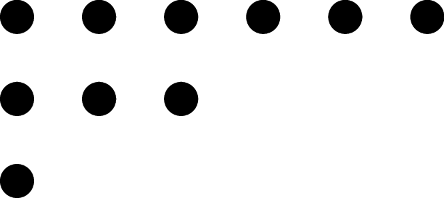
To represent a partition as a Ferrers diagram we draw a row of dots for each part in the partition and stack them from top to bottom in descending order, i.e. longest row/largest part at the top, aligned to the upper-left corner (of the 4th quadrant). For example, the Ferrers diagram for the partition $\lambda = (6,3,1)$ is given by
We can use the ferrers_diagram() method to return the Ferrers diagram of a partition as a string, and we can use the pp() method to print the Ferrers diagram to the display.
mu = Partition([6,3,1])
print(type(mu.ferrers_diagram()))
# <type 'str'>
mu.pp() # Runs print(mu.ferrers_diagram()), returns None
# ******
# ***
# *
Young diagrams and Young tableaux
A Young diagram is very similar to a Ferrers diagram except we draw rows of boxes instead of dots. For example, we display the Young diagram for the partition $\lambda = (6,3,1)$ below.
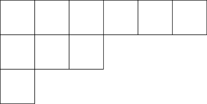
Young diagrams are a more useful way of visualizing partitions because we can fill the boxes (cells) with numbers (or other data) to obtain Young tableux.
Conjugation
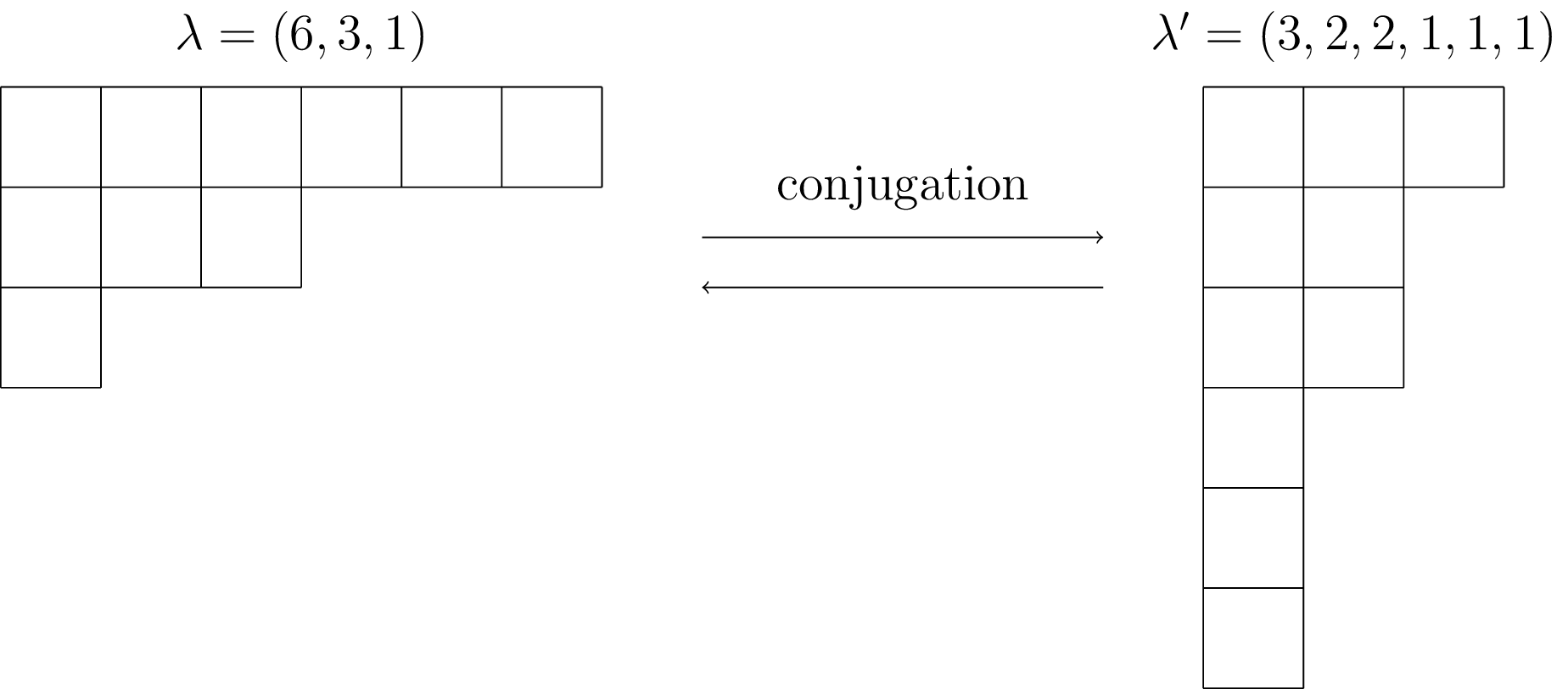
The conjugate of the partition $\lambda$ is the partition $\lambda’$ obtained by swapping the rows and columns in the Young diagram. Formally, $\lambda’(j):=|\{i:\lambda(i)\ge j\}|$ for each $j\in \mathbb{Z}_{>0}$. This is also called the associated partition or the transpose in the literature.
For example, if $\lambda = (6,3,1)$, then its conjugate is given by $\lambda’=(3, 2, 2, 1, 1, 1)$.
- Notice that conjugation is a size-preserving operation on the set of partitions. That is, $\mathrm{size}(\lambda’)=\mathrm{size}(\lambda)$.
- Notice that if we take the conjugate of a partition twice we get back the partition we started with. That is, $(\lambda^\prime)^\prime=\lambda$. Therefore conjugation is what is known as an involution, i.e. a self-inverse function, on the set of partitions.
We can calculate the conjugate of a partition in SageMath using the conjugate() method or the helper function of the same name.
Partition([5,5,3,2,1]).conjugate() # Same as conjugate(Partition([5,5,3,2,1]))
# [5, 4, 3, 2, 2]
Partition([5,5,3,2,1]).conjugate().conjugate() # Same as conjugate(Partition([5, 4, 3, 2, 2]))
# [5, 5, 3, 2, 1]
Cells
We call each box (resp. dot) in a Young (resp. Ferrers) diagram a cell in the diagram, with coordinates $(i,j)$ for the cell in the $i$-th row and $j$-th column of a partition. For a partition $\lambda=(\lambda_{1},\lambda_{2},\ldots,\lambda_{k})$ we identify its Young diagram with the set of cells $$\mathrm{Young}(\lambda) = \{(i,j)|1 \le i \le k, 1 \le j \le \lambda_{i}\}$$
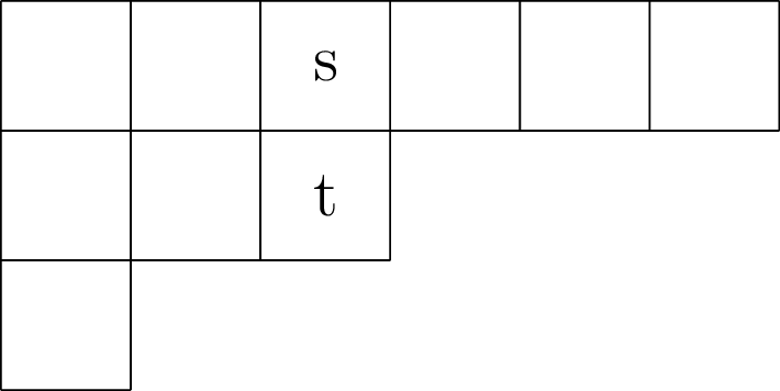
Let $\lambda = (6,3,1)$. We highlight the cells $s = (1,3), t = (2,3) \in \mathrm{Young}(\lambda)$ in the diagram below
We can obtain the coordinates of the cells in a partition as a list using the cells() method, but note that in Python/SageMath that indices are $0$-based (i.e. indices start from $0$ instead of $1$).
Partition([6,3,1]).cells()
# [(0, 0), (0, 1), (0, 2), (0, 3), (0, 4), (0, 5), (1, 0), (1, 1), (1, 2), (2, 0)]
It should be clear that the size of a partition $\lambda$ is equal to the number of cells in its Young diagram, that is $\mathrm{size}(\lambda) = |\mathrm{Young}(\lambda)|$, and that we can recover the parts of a partition from its Young diagram by counting the number of cells in the corresponding row: $\lambda_{i} = |\{(i,j)\in\mathrm{Young}(\lambda)\}| = \max\{j:(i,j)\in\mathrm{Young}(\lambda)\}$.
Given a partition $\lambda$, there is a canonical bijection between the cells in $\mathrm{Young}(\lambda)$ and those in $\mathrm{Young}(\lambda’)$ arising from the relation $(i,j)\in\mathrm{Young}(\lambda)\iff(j,i)\in\mathrm{Young}(\lambda’)$.
Arms, legs, and hooks
Given a cell $(i,j)$ in a Young diagram, we define the arm, leg, and hook of $(i,j)\in\mathrm{Young}(\lambda)$ as the following subsets of $\mathrm{Young}(\lambda)$:
$$ \mathrm{arm}_{\lambda}(i,j):= \{(i,y):j < y \le \lambda_i\}\subset\mathrm{Young}(\lambda)$$ $$ \mathrm{leg}_{\lambda}(i,j):= \{(x,j):i < x \le \lambda’_j\}\subset\mathrm{Young}(\lambda)$$ $$ \mathrm{hook}_{\lambda}(i,j):= \{(x,y):i < x \le \lambda’_j, j \le y \le \lambda_{i}\} = \mathrm{arm}_{\lambda}(i,j)\cup\mathrm{leg}_{\lambda}(i,j)\cup\{(i,j)\}$$
The arm of a cell $s=(i,j)$ consists of the cells on the same row of the Young diagram as $s$ which are further from the origin. Similarly, the leg of $s\in\mathrm{Young}(\lambda)$ consists of all cells in $\mathrm{Young}(\lambda)$ which lie on the same column, but further from the origin. Finally, $\mathrm{hook}_{\lambda}(s)$ is made up of all the cells from both the arm and leg of $s$ in $\lambda$ together with the cell $s$ itself.
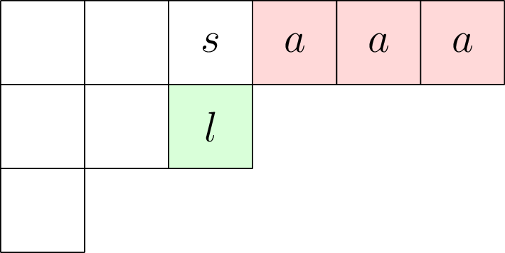
As an example, we let $\lambda = (6,3,1)$ and $s = (1,3)\in \mathrm{Young}(\lambda)$ and highlight cells in $\mathrm{arm}_{\lambda}(s)$ with the letter $a$ on a red background and cells in $\mathrm{leg}_{\lambda}(s)$ with the letter $l$ on a green background in the diagram below:
Given a partition $\lambda$, we can define associated functions $a_{\lambda},l_{\lambda},h_{\lambda}:\mathrm{Young}(\lambda)\to\mathbb{Z}_{\ge0}$, called the arm length, leg length, and hook length, respectively, which act on cells in the Young diagram of $\lambda$ as follows:
$$ a_{\lambda}(i,j):=\lambda_i - j $$ $$ l_{\lambda}(i,j):=\lambda’_j - i $$ $$ h_{\lambda}(i,j):= a_{\lambda}(i,j) + l_{\lambda}(i,j) + 1 $$
where $\lambda’$ is the conjugate partition to $\lambda$.
For $\lambda = (6,3,1)$, $s = (1,3)\in \mathrm{Young}(\lambda)$ as above, we find that $a_{\lambda}(s) = 6 - 3 = 3$, $l_{\lambda}(s) = 2 - 1 = 1$, $h_{\lambda}(s) = 3 + 1 + 1 = 5$.
As their names suggest, the functions $a_{\lambda},l_{\lambda},h_{\lambda}$ count the number of cells in the arm, leg, and hook of a cell, respectively, that is $a_{\lambda}(i,j)=|\mathrm{arm}_{\lambda}(i,j)|$, $l_{\lambda}(i,j)=|\mathrm{leg}_{\lambda}(i,j)|$, and $h_{\lambda}(i,j)=|\mathrm{hook}_{\lambda}(i,j)|$. In principle the functions $a_{\lambda},l_{\lambda},h_{\lambda}$ could be extended to the lattice $(\mathbb{Z}_{\ge0})^{2}\to\mathbb{Z}$ using the fact that $\lambda(i)=0$ for $i>\mathrm{length}(\lambda)$.
Table of functions
In the table below we recap the definitions from this subsection along with their implementations as methods for the Partition class in SageMath, as well as introducing a few other functions in passing. At this point we only remark that the functions for $\alpha$-upper hook length and $\alpha$-lower hook length are simply generalisations of the classical hook length discussed above and coincide when $\alpha=1$.
| Math notation | SageMath method | Description |
|---|---|---|
| $\mathrm{arm}_{\lambda}(i,j)$ | arm_cells(i,j) |
$\{(i,y):j < y \le \lambda_i\}$ |
| $\mathrm{leg}_{\lambda}(i,j)$ | leg_cells(i,j) |
$\{(x,j):i < x \le \lambda’_j\}$ |
| $\mathrm{hook}_{\lambda}(i,j)$ | hook_cells(i,j) |
$\mathrm{arm}_{\lambda}(i,j)\cup\mathrm{leg}_{\lambda}(i,j)\cup\{(i,j)\}$ |
| $a_{\lambda}(i,j)$ | arm_length(i,j) |
$\lambda_i - j = |\mathrm{arm}_{\lambda}(i,j)|$ |
| $l_{\lambda}(i,j)$ | leg_length(i,j) |
$\lambda’_j - i = |\mathrm{leg}_{\lambda}(i,j)|$ |
| $h_{\lambda}(i,j)$ | hook_length(i,j) |
$a_{\lambda}(i,j) + l_{\lambda}(i,j) + 1 = |\mathrm{hook}_{\lambda}(i,j)|$ |
| $\mathrm{Graph}(a_{\lambda})$ | arm_lengths() |
A Young tableau of $\lambda$ with cells filled in with their arm lengths |
| $\mathrm{Graph}(l_{\lambda})$ | leg_lengths() |
A Young tableau of $\lambda$ with cells filled in with their leg lengths |
| $\mathrm{Graph}(h_{\lambda})$ | hook_lengths() |
A Young tableau of $\lambda$ with cells filled in with their hook lengths |
| $h^{\ast}_{\lambda}(i,j;\alpha)$ | upper_hook(i,j,alpha) |
$\lambda^{\prime}_j - i + \alpha(\lambda_i - j + 1) = l_{\lambda}(i,j) + \alpha(a_{\lambda}(i,j) + 1)$ |
| $h_{\ast}^{\lambda}(i,j;\alpha)$ | lower_hook(i,j,alpha) |
$\lambda^{\prime}_j - i + 1 + \alpha(\lambda_i - j) = l_{\lambda}(i,j) + 1 + \alpha\cdot a_{\lambda}(i,j)$ |
| $\mathrm{Graph}(h^{\ast}_{\lambda}(\cdot;\alpha))$ | upper_hook_lengths() |
Tableau of $\lambda$ with cells filled in with their $\alpha$-upper hook lengths |
| $\mathrm{Graph}(h_{\ast}^{\lambda}(\cdot;\alpha))$ | lower_hook_lengths() |
Tableau of $\lambda$ with cells filled in with their $\alpha$-lower hook lengths |
mu = Partition([6,3,1])
mu.arm_cells(0,2) # Indices are zero-based
# [(0, 3), (0, 4), (0, 5)]
mu.leg_length(0,2) # Check above example
# 1
mu.hook_lengths() # Returns a list of lists
# [[8, 6, 5, 3, 2, 1], [4, 2, 1], [1]]
You can practice executing SageMath and Python code in the SageMathCell below.