Notation

Alternative notation

Besides thinking of partitions as a sequence of summands (parts), we may encode the data in a handful of other ways. This can be useful for computation, compactness, or for realizing the appearance of partitions in other areas of mathematics and beyond.

In fact, the cycle of discovery often begins with mathematicians studying an object of interest in their own field, only later realizing that after a little bit of manipulation the problem at hand can also be viewed in terms of partitions.

Exponential notation

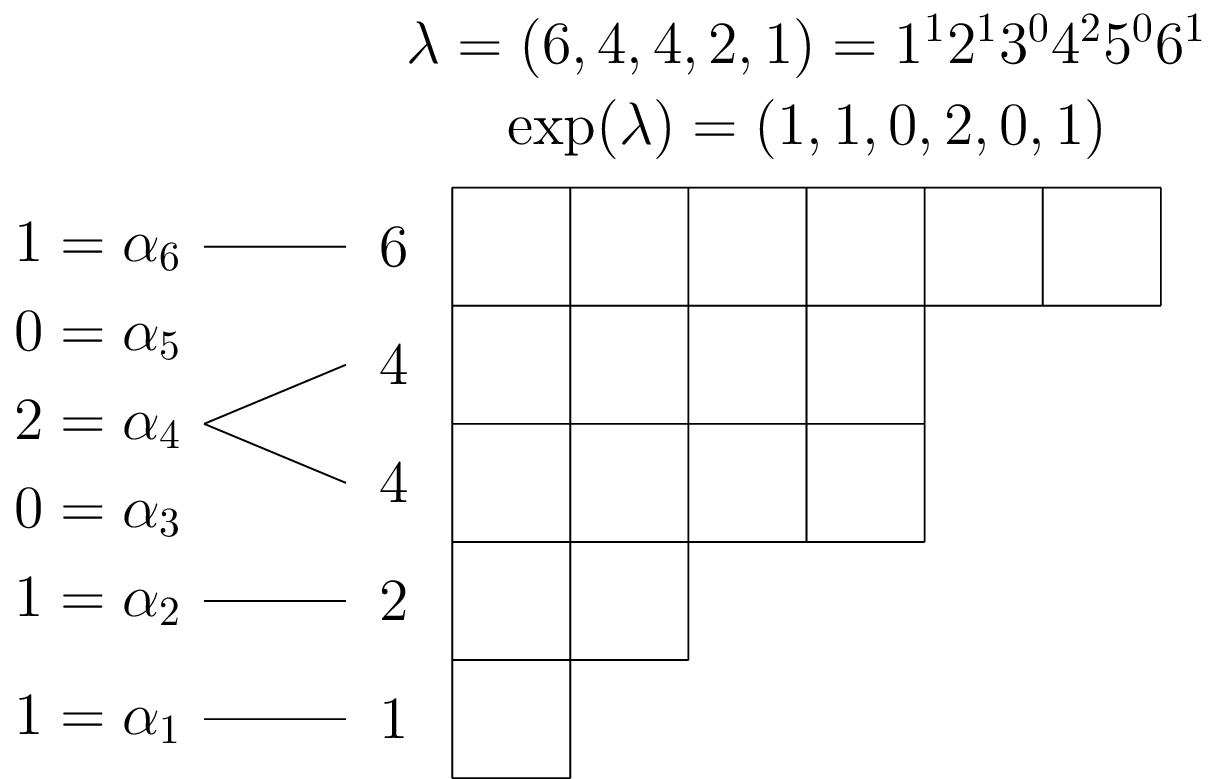
The most simple alternative to describing a partition $\lambda$ by listing its parts $\lambda_{j}$ is exponential notation, where instead we count the number of parts of size $i$ appearing in $\lambda$ for each positive integer $i$, that is $\alpha_{i}=|\{j\in\mathbb{Z}_{>0}|\lambda(j)=i\}|$, to form a finite sequence of nonnegative integers $\exp(\lambda):\mathbb{Z}_{>0}\to\mathbb{Z}_{\ge0}$ given by $\exp(\lambda)(i):=\alpha_{i}$.

We usually write this as $\lambda=1^{\alpha_{1}}2^{\alpha_{2}}3^{\alpha_{3}}\ldots\lambda_{1}^{\alpha_{\lambda_{1}}}$ where $\lambda_{1}=\max\{i\in\mathbb{Z}_{>0}|\alpha_{\lambda}(i)\ne0\}$ is called the largest part in $\lambda$, but may also directly write $\exp(\lambda)=(\alpha_{1},\alpha_{2},\alpha_{3},\ldots,\alpha_{\lambda_{1}})$. For example:

We can obtain the exponential notation for a given partition in SageMath using the to_exp() method, and we can construct a partition from its exponential form using the exp keyword argument in the constructor.

Partition([6,4,4,2,1]).to_exp()
# [1, 1, 0, 2, 0, 1]
Partition(exp=[1,1,0,2,0,1])
# [6, 4, 4, 2, 1]

Frobenius Coordinates

The Frobenius rank of a partition $\lambda$ is given by the number of cells on the main diagonal of $\lambda$, and formally defined to be $\max\{i\in\mathbb{Z}_{>0}:\lambda_{i}\ge i\}$. This is also equal to the length of the largest square fitting into the Young diagram of $\lambda$. For example, the Frobenius rank of the partition $\lambda = (6,4,4,2,1)$ is $3$.

We can obtain the Frobenius rank for a given partition in SageMath using the frobenius_rank() method.

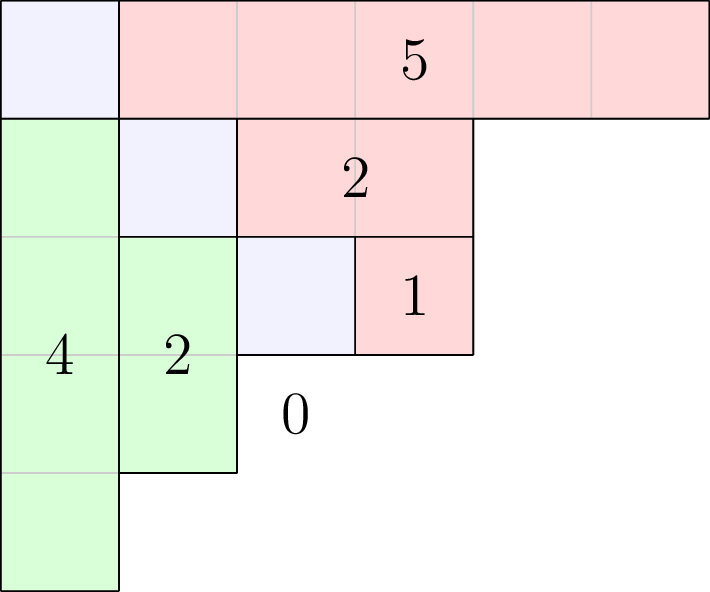
The Frobenius coordinates of a partition $\lambda$ of Frobenius rank $r$ is a pair of length-$r$ integer-valued vectors $p,q$ given by listing the arm and leg statistics, respectively, of the cells along the main diagonal in $\lambda$. That is, for $i=1,2,\ldots,r$

$$p_{i}=a_{\lambda}(i,i),q_{i}=l_{\lambda}(i,i).$$

For example, the diagram below illustrates how to obtain the Frobenius coordinates $p=(5,2,1)$, $q=(4,2,0)$ from the partition $\lambda = (6,4,4,2,1)$:

We can obtain the Frobenius coordinates for a given partition in SageMath using the frobenius_coordinates() method, and we can also construct a partition using the frobenius_coordinates keyword argument in the constructor.

Partition([6,4,4,2,1]).frobenius_coordinates()
# ([5, 2, 1], [4, 2, 0])
Partition(frobenius_coordinates=([5, 2, 1], [4, 2, 0]))
# [6,4,4,2,1]

Notice that if a partition $\lambda$ has Frobenius rank $r$, then for $i=1,2,\ldots,r-1$, its Frobenius coordinates $p,q$ must satisfy $p_{i+1}\le p_{i}-1$, and $q_{i+1}\le q_{i}-1$. That is to say, the Frobenius coordinates consist of strictly decreasing integer sequences of finite length.

If the Frobenius coordinates of a partition $\lambda$ is given by the pair $(p,q)\in\mathbb{Z}_{\ge0}^{r}\times\mathbb{Z}_{\ge0}^{r}$, then the Frobenius coordinates of its conjugate $\lambda’$ are given by the pair $(q,p)$. This follows from the deduction that $a_{\lambda’}(i,j)=l_{\lambda}(j,i)$, which we apply to the special case $i=j$, along with the bijection $\mathrm{Young}(\lambda)\to\mathrm{Young}(\lambda’)$ given by $(i,j)\mapsto(j,i)$ mentioned earlier.

Maya diagrams, zero-one sequences, and Dyck words

In this section we introduce Maya diagrams, and explain their connection to partitions, Dyck paths from combinatorics, and the physical model known as “Dirac’s electron sea”.

Maya diagrams are used to visualize binary sequences of zeros and ones, and the two states 0 and 1 can be used to represent a wide range of paired notions, such as two directions when traversing a binary tree, two vectors in a basis of a 2D lattice, or a pair of oppositely charged particles (e.g. electrons and positrons).

Minimal zero-one sequences

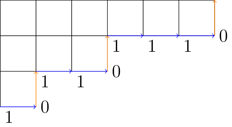
We begin by explaining the zero_one_sequence() method for partitions in SageMath. We draw the Young diagram of a partition in English notation and label edges on its outer rim/boundary path according to the rule North=0 and East=1, and then read this 0-1 sequence from $(0, -\infty)$ to $(+\infty, 0)$ so that part size increases as we read along the boundary path.

Though such a sequence starts with infinitely many 0s and end with infinitely many 1s, the zero_one_sequence() method omits these to return a finite output, describing only the edges on the boundary of the Young diagram which do not lie on the axes. This may be called the minimal 0-1 sequence of a partition.

Below we illustrate how to obtain the minimal zero-one sequence $(1,0,1,1,0,1,1,1,0)$ from the partition $\lambda=(6,3,1)$:

We can obtain the minimal zero-one sequence of a given partition in SageMath using the zero_one_sequence() method, and we can also construct a partition using the zero_one keyword argument in the constructor.

Partition([6,3,1]).zero_one_sequence()
# [1, 0, 1, 1, 0, 1, 1, 1, 0]
Partition(zero_one=[1,0,1,1,0,1,1,1,0]) # Same as Partitions().from_zero_one([1,0,1,1,0,1,1,1,0])
# [6,3,1]

This leads to reading boundary paths from right to left in Russian and Cartesian notations.

Dyck words

Next we explain the to_dyck_word() method for partitions in SageMath. We draw the Young diagram of a partition in English notation and label edges on its outer rim/boundary path according to the rule North=1 and East=0, and then read this 0-1 sequence from $(0, -\infty)$ to $(+\infty, 0)$ so that part size increases as we read along the boundary path.

We will begin with an illustration of how to obtain the Maya diagram corresponding to a given partition before discussing the formal definitions and details. Just as with Young diagrams, Maya diagrams are also subject to choices of convention for how they relate to a particular partition, but for our purposes, we will fix the following convention:

We can obtain the Dyck word associated to a given partition in SageMath using the to_dyck_word() method, and we can also recover the partition from its Dyck word using the to_partition() method.

Partition([6,3,1]).to_dyck_word()
# 
Partition([6,3,1]).to_dyck_word(10)
# 
Partition([6,3,1]).to_dyck_word().to_partition()
# [6,3,1]

States

Consider the set of integers $\mathbb{Z}$ as the disjoint union $\mathbb{Z}=\mathbb{\mathbb{Z}}_{<0}\sqcup\mathbb{Z}_{\ge0}$ of the negative integers $\mathbb{Z}_{<0}$ and the nonnegative integers $\mathbb{Z}_{\ge0}$. We define a state to be a subset $S\subset\mathbb{Z}$ such that the symmetric difference $S\Delta\mathbb{Z}_{\ge0}$ is finite. That is, for $S^{C}:=\mathbb{Z}\setminus S=\{n\in\mathbb{Z}|n\notin S\}$

$$ S\Delta\mathbb{Z}_{\ge0}=(S\setminus\mathbb{Z}_{\ge0})\sqcup(\mathbb{Z}_{\ge0}\setminus S)=(S\cap\mathbb{Z}_{<0})\sqcup(S^{C}\cap\mathbb{Z}_{\ge0})\,\text{finite.} $$

We may identify a state $S\subset\mathbb{Z}$ with the pair of (necessarily) finite sets $(S\cap\mathbb{Z}_{<0})$ and $(S^{C}\cap\mathbb{Z}_{\ge0})$ by the bijection between

$$ \{S\subset\mathbb{Z}|S\Delta\mathbb{Z}_{\ge0}\,\text{finite}\} \leftrightarrow \{(A,B)|A\subset\mathbb{Z}_{\ge0}\,\text{finite},B\subset\mathbb{Z}_{<0}\,\text{finite}\} $$

given by $S\mapsto(S^{C}\cap\mathbb{Z}_{\ge0}$, $S\cap\mathbb{Z}_{<0})$, with inverse given by $(A,B)\mapsto A^{C}\cap(B\cup\mathbb{Z}_{\ge0})$.

Zero-one sequences

A Maya diagram is a function $\mathrm{\boldsymbol{m}}:\mathbb{Z}\to\{0,1\}$ such that there exist $N,M\in\mathbb{Z}$ such that for all $\nu>N$ we have $\boldsymbol{\mathrm{m}}(\nu)=1$ and for all $\nu<M$ we have $\boldsymbol{\mathrm{m}}(\nu)=0$. It follows that $M\le N+1$.

Let $S\subset\mathbb{Z}$ be a state, then its identity function $\mathbb{1}_{S}:\mathbb{Z}\to\{0,1\}$,

$$\mathbb{1}_{S}(\nu) = \begin{cases} 1 & \nu\in S\\ 0 & \nu\notin S \end{cases}$$

is a Maya diagram, where we may take $N=\max(S^{C}\cap\mathbb{Z}_{\ge0})$, $M=\min(S\cap\mathbb{Z}_{<0})\in\mathbb{Z}$.

On the other hand, for a Maya diagram $\mathrm{\boldsymbol{m}}:\mathbb{Z}\to\{0,1\}$ we may define a state $S=\boldsymbol{\mathrm{m}}^{-1}(1)=\{\nu\in\mathbb{Z}|\boldsymbol{\mathrm{m}}(\nu)=1\}$, in which case

$$ |S\cap\mathbb{Z}_{<0}|=|\{\nu\in\mathbb{Z}_{<0}|\mathrm{\boldsymbol{m}}(\nu)=1\}|\le\max(0,-M) $$

and

$$ |S^{C}\cap\mathbb{Z}_{\ge0}|=|\{\nu\in\mathbb{Z}_{\ge0}|\boldsymbol{\mathrm{m}}(\nu)=0\}|\le\max(0,N+1).$$

We define the charge of a Maya diagram/state to be the difference

$$ \mathrm{charge}(S)=|S^{C}\cap\mathbb{Z}_{\ge0}|-|S\cap\mathbb{Z}_{<0}|=|\boldsymbol{\mathrm{m}}^{-1}(0)\cap\mathbb{Z}_{\ge0}|-|\boldsymbol{\mathrm{m}}^{-1}(1)\cap\mathbb{Z}_{<0}|.$$

Beta numbers

Beta numbers have applications in Representation theory.

Interchanging between notations

We can prove that these notations are equivalent and that we can freely interchange between them, i.e. that the set of partitions is in bijection with the set of e.g. Frobenius coordinates

We also demonstrate and explain how these have been implemented in SageMath

# Insert code here